Statistics for Machine Learning

"By Statistics, we mean methods specially adopted to the elucidation of quantitative data affected to a marked extent by multiplicity of causes. --Yule and Kendal

It is different from Business Analytics that can be defined as:

Business Analytics (BA) can be defined as the broad use of data and quantitative analysis for decision making within organizations. -- Thomas Davenport

Statistics is broadly divided into two categories:

1. Descriptive
2. Inferential

Descriptive Statistics involves describing the data, summarising information from the data, and providing a convenient overview to the data in a brief. It is like online dating: it is definite but can be misleading.

For example, if we try to answer the question who is the best batsman in the world of all time in cricket, then there can be many factors to determine this which leads to a confusion. Descriptive statistics based approach may involve say taking the average of all the scores by a batsman and providing it as a single convenient value to evaluate the performance of batsman. This helps in visualising the data in layman terms to provide a definitive perspective to the users.

Inferential Statistics involves learning to make a prediction from the given data or extract information with unusual patterns that can prove to be useful in decision making. It is concerned with population parameters from a sample.

For example, studying the stock market prices in order to predict the prices of the future, and perform risk analysis in order to determine the optimal amount to be invested to maximise profits and prevent loss of investments.

There is also a third category called 'Prescriptive Statistics'. This is used in presribing the test subject with a treatment to affect behaviour of the subject and observe the results to get better interpretations that can be applied to the population.

For example, a doctor treating a set of patients with a certain illness and he tries different treatment to each patient for a week to observe how they react to the treatment, and whichever gets the best results then that treatment is recommended or 'prescribed' to the others who are having similar symptoms.

Data Types

The first major form of different types of data is in terms of structured and unstructured data. We are concerned with structured data more that has an organized nature and can be used to extract meaningful information and extract patterns from it.

A broad distinguishing feature of data is in terms of its measurement.

• Qualitiative: The data that is non-numeric by nature and cannot be measured is called qualitative data.
• Quantitative: The data that is numerical by nature and is measurable is called quantitative data. It can be classified into discrete and continous types of data.

Hence, we will now get into details of the different types of such data.

• Continous: Data that can take on any interval
• Discrete: Data that can take on any integer value
• Categorical: Data that can take a specific set of values representing a set of possible categories
• Binary: Data with only two possible categories or values ie 0/1 or True/False
• Ordinal: Categorical Data that has explicit ordering

Examples:

• Continous Data: Wind speed, time durations
• Discrete Data: Count of occurences of an event, number of persons in a population
• Categorical Data: List of states in a country
• Binary Data: Gender: Male or Female, Email Spam/not Spam
• Ordinal Data: T-shirt sizes: S, M and L

Why do we need to classify data into different types?

• Storage and indexing can be optimized
• The possible values of a categorical variable can be enforced in a software (eg. enum)
• Knowing the nature of the data can help us plot a visual or fit a model

Key Terms in Statistics

1. Population: The total number of possible data points present in the data is called its population.
2. Sample: A subset of the population selected in such a way that it preserves the variance of the population and exhibits same behaviour when subjected to operations much like the overall population.
3. Statistic: It is a numerical value associated with an observed sample.
4. Parameter: It is a numerical value associated with a population.

Now, why are we learning statistics?? Our aim is to get information from raw data.

Raw Data represent numbers and facts in the original format in which the data have been collected. We need to convert the raw data into information for decision making.

When we mine useful patterns after structuring this data, we get the data in form of information.

Estimates of Location

1. Mean: The sum of all values divided by the number of values.
2. Weighted Mean: The sum of all values times the weight of each observation in the data.
3. Median: The middle value of data, in case of even number of terms we take the average of the two middle values present in the data.
4. Weighted Median: The value such that one half of the sum of weights lies above and other half lies below the sorted data.
5. Trimmed Mean: The average of all the values after dropping a fixed number of extreme values.
6. Robust: Not sensitive to extreme values.
7. Outlier: A datapoint which exhibits different behaviour from the majority of data points in the population.

Mean = where N = Total number of records or Population n = Total number of records in Sample and n is a subset of N

• Note: Mean is known to be prone to outlier or extreme values For example, we are calculating the average of incomes of persons sitting in a restaurant with lowest income being $100 and highest being $500, and mean income is nearly about $300. Suddenly, Bill Gates enter the restaurant and takes a seat. His income is $1 billion (assume), so now the new mean will be approximately a billion which is way higher than incomes of others in the same dataset or population. Hence, mean is sensitive to outliers.

• Thus, we use a trimmed mean as described which drops these extreme values. Trimmed Mean = where p are the extreme values on both sides of the data.

• Weighted Mean = / is used when the data does not represent all the groups equally and some variables are more intrinsic than other variables and need to be given higher weights as a result.

• Median:

  • Sort the values in ascending order
  • If the number of terms is odd, then take the middle value
  • If the number of terms is even, then take the average of the middle values
    Median is a robust estimate because it is not affected by outliers

Notebook for Measures of Central Tendency: Link

Estimates of Variability and Percentiles

1. Deviations: The difference between the observed values and estimates of location.
2. Variance: The sum of squared deviations from the mean divided by n-1 where n is the number of data points.
3. Standard Deviation: Measure of dispersion within the data which is square root of variance.
4. Range: The difference between the maximum and minimum value in the data.
5. Percentile: The value of P percent of the values take the value less than or this and (100-P) percent takes on this value or more.
6. Interquartile Range: The difference between 75th percentile and the 25th percentile is the IQR.

Mean Absolute Deviation = 1/n

Standard Deviation =

Variance =

Degrees of Freedom

1. We make use of n-1 terms and not all of n terms in calculating variance.
2. If we use n terms in the denominator we end up having a biased estimate. However, if we divide by n-1 terms, the standard deviation becomes an unbiased estimate.
3. The reason for the biased estimate in case of n terms are considered is that the mean also considers n number of terms and is present in the formula.

A robust estimate of variability is the median absolute deviation (MAD). MAD = Median() where Standard Deviation > Mean Absolute Deviation The range is given as follows:

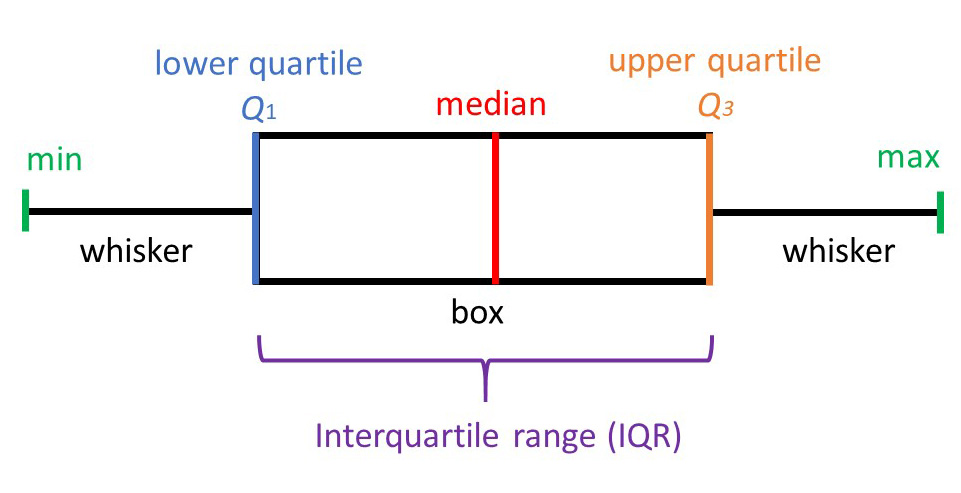
Further, we divide the data into four quarters as follows:

1. Lower Quartile (Q1): It is the quarter of data with the lowest values.
2. Upper Quartile (Q4): It is the quarter of data with highest values.
3. Interquartile Range (Q3-Q1): The difference between the 75th percentile and 25th percentile of the data.

IQR is the middle half of the data, which is not susceptible to outliers making it most suitable for dealing with skewed distributions.

When you have a skewed distribution, the median is a better measure of central tendency, and it makes sense to pair it with either the interquartile range or other percentile-based ranges because all of these statistics divide the dataset into groups with specific proportions.

For normally distributed data, or even data that arent terribly skewed, using the tried and true combination reporting the mean and the standard deviation is the way to go. This combination is by far the most common. You can still supplement this approach with percentile-base ranges as you need.

Notebook for Measures of Variability: Link

Exploring Data Distributions and Visualizations

Pandas provides a simple five-point summary of the data that gives insight to different aspects:

1. X(smallest)
2. First Quartile (Q1)
3. Median (Q2)
4. Third Quartile (Q3)
5. X(largest)
   This is captured most beautifully by a visualization of distribution called Boxplot.

• Boxplot: It is a quick way to visualize the distribution of the data with the five point summary.

  • A value is considered to be an outlier if it falls at 1.5 times the interquartile range below Q1 or above Q3.
  • The boxplot of a symmetric distribution has the median in the middle with equally spaced out data on both the sides
    

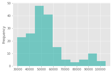
• Frequency Table or Histograms: It is a frequency distribution of the data, and they are stacked together using bins. If they are too small, the result will be granular and the ability to see bigger pictures are lost.

  • X-axis: Bins
  • Y-axis: Count
  • They show the exact data distribution along with the variance in the data which is absent in boxplot.
    

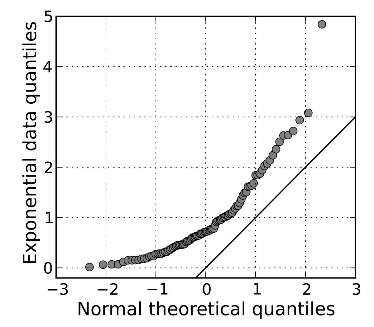
• Quantile Plot: Displays all of the data (allowing the user to assess both the overall behavior and unusual occurrences)

  • Plots quantile information
  • For a data x(i) data sorted in increasing order, f(i) indicates that approximately 100 f(i) % of the data are below or equal to the value x(i)
    

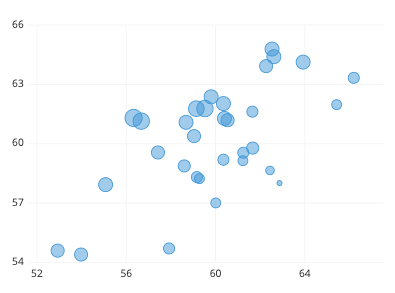
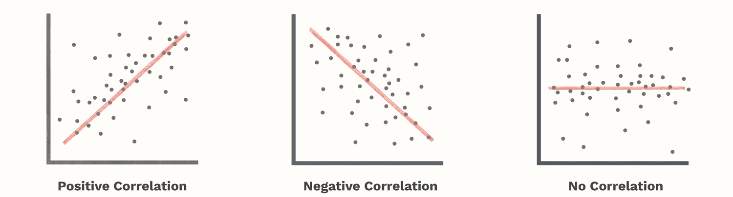
• Scatter Plot: It shows the direct relationship between the dependent and independent variables in the data.

Correlations and Covariance

Correlations refers to simple idea of determining relationship between a set of features, and it can be simply seen as the following possibilities:

1. A feature increases, with corresponding increase in other feature.
2. A feature decreases with corresponding decrease in other feature.
3. A feature increases, with corresponding decrease in other feature.
4. A feature decreases, with corresponding increase in other feature.
   And yes we might also have no effect of changing values of one feature on another which means that both the features being compared are independent of each other.

• Correlation quantifies how much two variables are associated with each other, but does not give the exact direction of this association.
• It can simply be defined as a measurement of association between two variables.
• It is highly sensitive to outliers.
• It can only capture linear relationships between two variables.

A fun example can be the amount of time you study and your GPA. A natural belief of people would be the more you study, the more marks should you get and hence a higher GPA, but most surveys and samples prove that if you study too much then your GPA is actually low compared to candidates who study for lesser hours but score more. Now, this is ofcourse subject to interpreting that there are many other factors associated with the example and not to mention the variance involved in the concentration of different students. But, the idea of correlation is to find unusual patterns, say as weird as the cost of a car wash and the time it takes to buy soda from the car wash station! That is when the actual data analysis comes into picture.

• Positive Correlation Coefficient: When a variable increases with corresponding increase in the other variable it is being compared with, the coefficient of correlation becomes positive.
• Negative Correlation Coefficient: When a variable increases with corresponding decrease in the other variable or vice versa then the coefficient of correlation becomes negative.
• Zero Correlation: There is no relationship between both the variables and they are independent of each other.
  
  Pearson Coefficient of Correlation =

However, actually we have Covariance as the numerator of this coefficient. Covariance tells us how much variability is present in the data from the mean and how much far is the data point from the mean. It does not tell us about the direction of the relationship but provides a quantifying measurement of the strength of association. Covariance(x,y) =

Hypothesis Testing

Hypothesis is an assumption about the population parameter to test whether the sample selected is a generic representation of the entire population. Hypothesis Testing simply refers to the process of decision making in order to accept or reject the hypothesis.

Why is Hypothesis required for analyzing data?

The population can be a very large dataset, hence making it computationally expensive to train on the entire data at once, hence we make use of sampling. Sampling is the process of selecting a subset of the data, which is an appropriate representative of the entire data so that when we run a model on this subset it can generate results that can be generalized on the entire population. There are two types of sampling available for any data:

1. Probability based Sampling
2. Non-Probability based Sampling

• Probability Sampling refers to the technique of sampling where each data point is given an equal chance of being selected in the sample from the population.

  • Simple Random Sampling refers to randomly selecting data points out of the population for a sample and trying out it for making a generalized model.
  • Systematic Sampling is the technique in which the first data point will be selected randomly followed by selecting points at 'n' intervals each.
  • Stratified Random Sampling refers to dividing the data into multiple subsets or groups and then selecting a random data point from each subset of the data to form the sample.
  • Cluster Sampling refers to treating each subset of data as a cluster and selecting that cluster as a sampling unit for analysis.

• Non-Probability based sampling does not give an equal chance to every data point

  • Convenience Sampling refers to the easiest method of sampling where we select data points based on their availability status and willingness to participate in an experiment.
  • Quota sampling refers to using a general criterion to filter out sample points and select those points from the population which fulfills the criterion.
  • Judgement Sampling refers to selecting the points by yourself and has the chance to be biased.
  • Snowball Sampling allows the points to randomly select their own further points for the sample from the population.
    There are two basis for a hypothesis formulation:

1. The NULL Hypothesis (): This states that the assumption made yields favourable results only by pure random chance.
2. The Alternate Hypothesis (): This states that the assumption made yields favourable results not by a pure random chance but by non-random cause.

Our goal is to reject the and accept the . There are many statisticians who argue that there is nothing called as 'Acceptance' because we cannot accept a NULL Hypothesis, there is either rejection of or we fail to reject the . From a simple perspective, the process of Hypothesis Testing has four broad steps:

1. State the and which must be mutually exclusive from each other which means that if one of them is True then the other one is definitely False.
2. Make an analysis plan, and describe how to evaluate the null hypothesis. The evaluation often focuses on a single test statistic.
3. Analyze the sample data using the appropriate chosen statistic whether it is mean, median or something else.
4. Interpret the results, as usual and apply the decision rule to the result to decide whether the task failed to reject the null hypothesis or rejected it successfully proving the alternative hypothesis.

Hypothesis Testing plays an integral part in deciding whether the assumptions made by the data scientist are correct or just random by chance on any data regarding patterns present in them. We come across different errors based on decision taken. In a summary, we can say that hypothesis testing is a kind of inferential statistics, where we try to prove an assumption for the entire population through a generated subset called sample of observations from within the population. A good example to understand the idea of hypothesis testing is as follows: Consider the example of trying to determine the percentage of community spread, in Bangalore with the rising number of COVID-19 cases. The Health Minister of Karnataka says that on average there is a 75% spread in infection cases. However, we cannot simply agree without proof, so here we are!

: The mean percentage of COVID-19 spread is 75% in Bangalore, Karnataka /: The mean percentage of COVID-19 spread is not 75% in Bangalore, Karnataka where is mean percentage is not equal to 75%

Now, we will perform the Z-Test: Z = where = Sample Mean, =Hypothesized Population Mean, =Standard Error/Deviation and n=Sample Size Through this, we are standardizing the sample mean we got. So if the sample mean is close enough to hypothesized mean , then Z will be close to 0. and we will have to accept the Null Hypothesis. Now, coming to how to reject it! So, we have to determine how big Z-value should be in order to reject the Null Hypothesis! Thus, we carry out a two-tailed distribution test, _ which is generally used when the hypothesis involves sign of equality or inequality_ 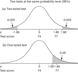Hence, we can define the two tailed test as follows: A two-tailed test is a test of a statistical hypothesis, where the region of rejection is on both sides of the sampling distribution and the region of acceptance is in the middle. The shaded parts in the given tests, are the Rejection Regions. The threshold values depends on the Significance Level taken for the hypothesis to be true. For example, we have =0.05 then the threshold values on two sides of a 2-tailed test will be 0.05/2 = 0.025 and then look this value in the Z-table, we find that Z-value is 1.96 and -1.96 so that will be the threshold on either sides. Therefore, the value of Z we get from the test is lower than -1.96, or higher than 1.96, we will reject the null hypothesis. Otherwise, we will accept it. Now, it can turn out that your hypothesis results will be wrong in terms of decision making. Thus, in general, two types of errors can arise:

1. Type-I Error (FALSE POSITIVE): This error arises when the Null Hypothesis is TRUE and we REJECT it.
2. Type-II Error (FALSE NEGATIVE): This error arises when the Null Hypothesis is FALSE and we ACCEPT it.
   For example,
   Consider the case of the following hypotheses:
   : The patient diagnosed has COVID-19
   : The patient diagnosed does not have COVID-19
   In this case we have two possibility of errors,

• The person has COVID-19 and is diagnosed to not have COVID-19 (FALSE POSITIVE or Type-1).
• The person does not have COVID-19 and is diagnosed to have COVID-19 (FALSE NEGATIVE or Type-2).

Now, before further we have to understand the concepts of Point Estimate in terms of Sample Mean () and Population Mean () with context to Hypothesis Testing.

• Point Estimate: It is located exactly in the middle of the confidence interval, so for example if we are talking about the Sample Mean, it is in the middle of the range covered for calculating the Population mean, similarly the same goes for the standard deviation of the sample with respect to that of the population.
• Confidence Interval: The range in which the population parameter is expected to be. It is defined as 1- where it indicates the confidence of finding the parameter within that range.
  For example, consider the case that the number of COVID-19 cases in a containment zone are 15. The local medical body is 90% confident to find the cases in that zone which means that =10%.

Also, we can say that the reader is interested in pursuing machine learning later in general considering you are looking for Statistical Insights to build concept, and I am 90% confident that you will learn machine learning after going through this curated content!

Now, coming to the concept where we do not want to perform hypothesis testing on the basis of predefined significance levels, and hence we make use of a p-value. This is the smallest significance value that can still reject the NULL hypothesis.

HOW TO CALCULATE THE P-VALUE? We calculate p-value, by the following formulae after calculating the Z-value of the sample:

• One-Tailed Test: (1 - Z-value corresponding in table) for one side
• Two-Tailed Test: (1 - Z-value corresponding in table)*2 for two sides
  For example, consider that we get a Z-value of 3.71, then look up in the Z-table, we get 0.4991! Hence, we get p-value = 1-0.499 which is approximately 0.5 > 0.025 that is the assumed value, now we cannot reject the NULL hypothesis, since the p-value is not higher than the value.
  Thus, for rejecting the NULL Hypothesis, the p-value should be smaller than the significance level otherwise it fails to reject the NULL Hypothesis.

So, let us see a simple difference between Z-Test and T-Test:

• Z-test is used when the sample test size is greater than 30, while T-test is more suitable for sizes less than 30.
• Z-test is used when we know the Population Standard Deviation, T-test is used when we do not know the Population Standard Deviation.
• Z-test is based on calculating the Z-value, while T-test takes account of the sample size too.

So, before we proceed any further let us be clear about all these tests and when to use them:

• ONE-SAMPLE TESTS: SAMPLE is being compared to POPULATION
• TWO-SAMPLE TESTS: TWO SAMPLES are being compared to each other
• PAIRED-SAMPLE TESTS: When the two samples being compared have variables that cannot be controlled
• F-TESTS: When more than two groups are being compared to each other
  Also, in a nutshell:
• t-Test: Any statistical hypothesis test in which the test statistic follows a Students t-distribution if the null hypothesis is supported.
• z-test: Any statistical test for which the distribution of the test statistic under the null hypothesis can be approximated by a normal distribution.

Simple Linear Regression

The Simple Linear Regression is a method to determine linear relationship between a dependent variable and independent variable(s). In simple words, if the independent variable increases then dependent variable also increases, and vice versa if it decreases.

The major difference between correlation and regression is that the correlation is a measure of strength of association between two variables, while regression quantifies this relationship.

A few key terms in describing the regression are:

• Independent Variables: The variables used to predict the response variable.
• Dependent Variable: The variable which has to be predicted using independent variables.
• Record: The vector of predictor and outcome values for a specific individual or case.
• Intercept: The predicted variable when X=0 on the line (b0).
• Regression Coefficient: The slope of the regression line (b1).
• Fitted Values: The estimates (y(i)) found on the regression lines.
• Residuals: The difference between the observed and predicted values.
• Least Squares: The method of fitting a regression line by minimizing the sum of squared residuals.

The Regression Equation is as follows:

y = b0 + b1.x

If the fitted values do not predict correctly (that is they do not fall on the line of regression) we compute residuals, which is used to be minimized in order to compute an extra error term explicitly.

y = b0 + b1.x + e

Residual Sum of Squares =

The method of minimizing the sum of residual squares is called the Ordinary Least Squares Regression (OLSR).

Till now, we discussed how the linear relationships are determined using regression and there is a non-linear aspect to regression to this.

Profiling: It is the term used to describe the relationship between prediction and explanation. A regression model can act as a predictive model and give us the values which are needed as the prediction of input features. However, it does not give us an explicit explanation of why this prediction is correct or not. This is done by our own knowledge.

For example, we can predict the number of purchases based on the number of ad clicks on a website but in the end it is our marketing knowledge that will tell us whether the sales increased and was profitable or not and not the other way around. This is called Profiling.

Hence, we can conclude that A regression model that fits the data well is set up such that changes in X lead to changes in Y. However, by itself, the regression equation does not prove the direction of causation. Conclusions about causation must come from a broader context of understanding about the relationship.

Thus, we come across three types of modelling in total as follows:

1. Predictive Modelling: The process of applying a statistical model or data mining algorithm to data for the purpose of predicting new or future observations.
2. Descriptive Modelling: Fitting a regression model can be descriptive if it is used for capturing the association between the dependent and independent variables rather than for causal inference or for prediction.
3. Explanation Modelling: A regression model can be explanatory if it is used to associate models for getting the causality behind the relationships of the dependent and independent variables.

Multiple Linear Regression

When multiple predictors are combined to get a single strong predictor as regression line then we refer to it as multiple linear regression.

It can be simply be represented as:

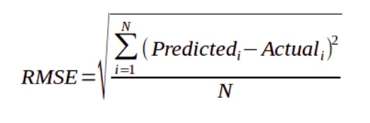
y = b0 + b1.x + b2.x2 + b3.x3 +.....+ bnxn + e where e is the root mean square error term.

Key Terms for Multiple Linear Regression:

1. Root Mean Squared Error (RMSE): The average squared error of regression is called Root Mean Square Error (RMSE).
   
2. Residual Square Error: The same as the root mean squared error, but adjusted for degrees
   of freedom.
3. R-Squared: The proportion of variance explained by the model, from 0 to 1.
4. t-statistic: The coefficient of predictor variable divided by the standard error, is a metric used to measure the statistical importance of the independent variables with respect to the response variable.
5. Weighted Regression: The terms have different weights that is number multiplied with the input predictors in order to get a regression line.

If we replace the denominator term in RMSE with n-p-1 then it is called Residual Standard Error and it is the basis for degrees of freedom.